Ideal time and message cost analysis for Mega-Merger: comparing theoretical results with empirical simulations

[ ]:

%matplotlib inline

from pydistsim.demo_algorithms.santoro2007.mega_merger.algorithm import MegaMergerAlgorithm, ExampleParameters
from pydistsim.benchmark import AlgorithmBenchmark
from pydistsim.network.behavior import NetworkBehaviorModel

Benchmarking: ideal communications

For this part, we will run a battery of simulations with the help of the benchmark module.

The parameters we will use are:

The algorithm to test.
The sizes of the networks to test.
The number of simulations to run for each network configuration (1 for now).
The network behavior (ideal communications obviously).

[3]:

from collections import defaultdict


benchmark_ideal = AlgorithmBenchmark(
    ((MegaMergerAlgorithm, ExampleParameters.numerical_parameters),),
    network_behavior=NetworkBehaviorModel.IdealCommunication,
    network_sizes=list(range(1, 30)) + list(range(30, 100, 10)) + list(range(100, 501, 50)),
    network_repeat_count=defaultdict(lambda: 1),  # 1 run for every network configurations
)

benchmark_ideal.run()

After the benchmark terminates, we can plot the results. But first, lets take a look at the raw data so we can understand what we may achieve.

[4]:

benchmark_ideal.get_results_dataframe(grouped=True)

[4]:

	Net. node count	Network type	Net. edge count	Qty. of messages sent	Qty. of messages delivered	Qty. of status changes	Qty. of steps
0	1	complete	0	0.0	1.0	4.0	3.0
1	1	homogeneous	0	0.0	1.0	4.0	3.0
2	1	hypercube	0	0.0	1.0	4.0	3.0
3	1	rectangular mesh	0	0.0	1.0	4.0	3.0
4	1	rectangular torus	1	1.0	2.0	7.0	5.0
...	...	...	...	...	...	...	...
260	483	rectangular mesh	802	8964.0	9146.0	10833.0	1215.0
261	500	complete	124750	256830.0	257033.0	339751.0	1423.0
262	500	homogeneous	10422	28268.0	28472.0	32991.0	447.0
263	500	ring	500	9337.0	9536.0	10145.0	2634.0
264	500	star	499	3112.0	3304.0	4805.0	4260.0

265 rows × 7 columns

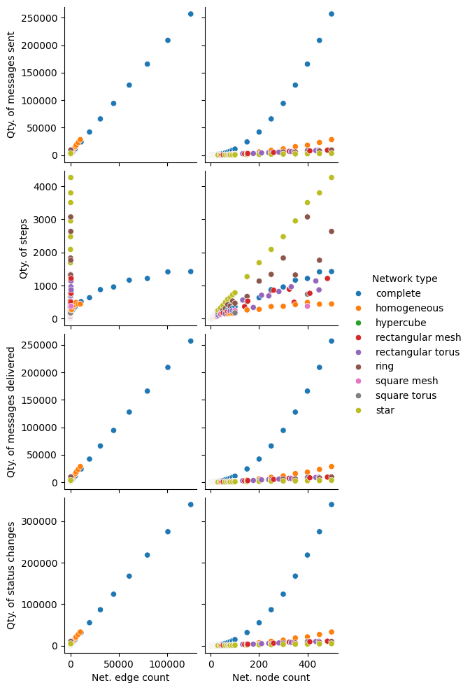
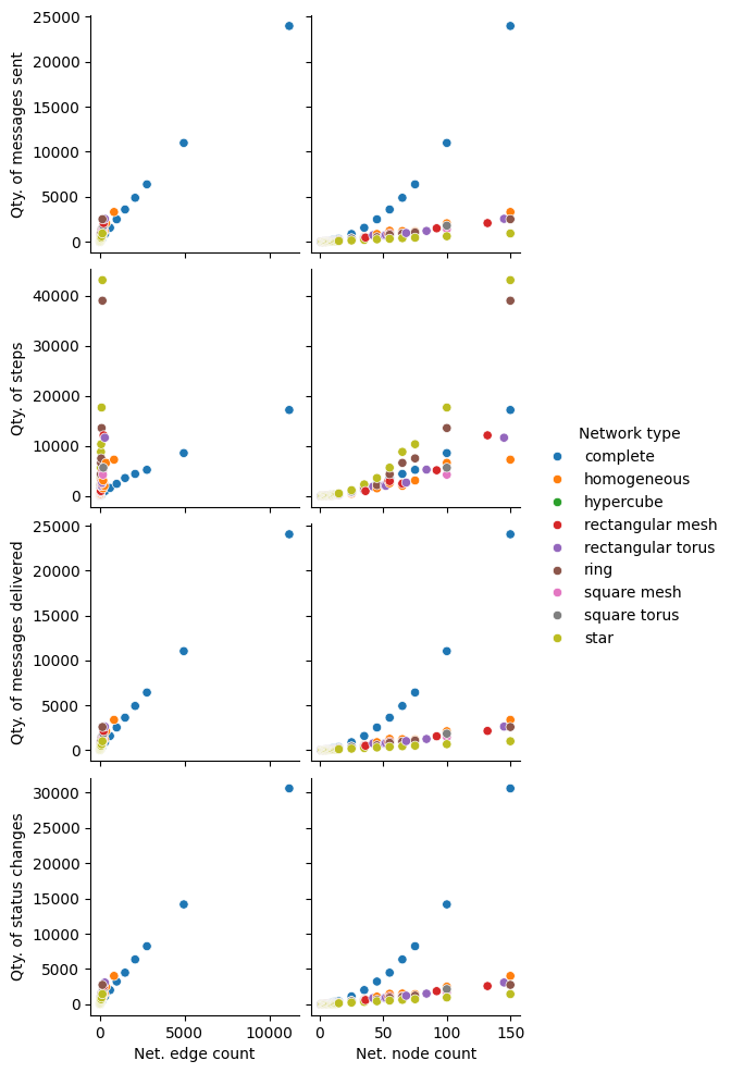
Plot everything:

[5]:

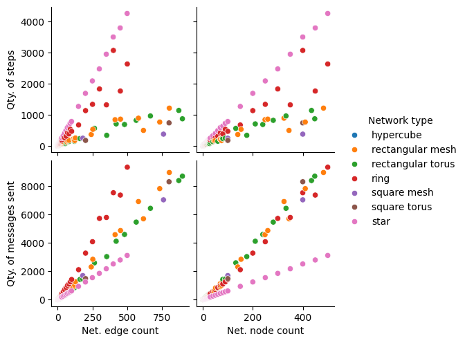
benchmark_ideal.plot_analysis()

[5]:

<seaborn.axisgrid.PairGrid at 0x7f153ba8aa10>

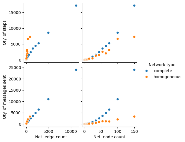
../../_images/notebooks_mega_merger_benchmarking_7_1.png

Plot only complete network results

Since the complete and homogeneous network results are the most interesting, we will plot them separately.

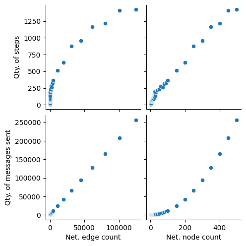
Complete network runs

[6]:

benchmark_ideal.plot_analysis(
    result_filter=lambda line: line["Network type"] == "complete", y_vars=["Qty. of messages sent", "Qty. of steps"]
)

[6]:

<seaborn.axisgrid.PairGrid at 0x7f153966e5d0>

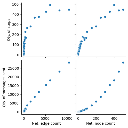
../../_images/notebooks_mega_merger_benchmarking_10_1.png

Homogeneous network runs

[7]:

benchmark_ideal.plot_analysis(
    result_filter=lambda line: line["Network type"] == "homogeneous", y_vars=["Qty. of messages sent", "Qty. of steps"]
)

[7]:

<seaborn.axisgrid.PairGrid at 0x7f153b9c5910>

../../_images/notebooks_mega_merger_benchmarking_12_1.png

Every other network type

[8]:

benchmark_ideal.plot_analysis(
    result_filter=lambda line: line["Network type"] not in ("complete", "homogeneous"),
    y_vars=["Qty. of messages sent", "Qty. of steps"],
)

[8]:

<seaborn.axisgrid.PairGrid at 0x7f1538223310>

../../_images/notebooks_mega_merger_benchmarking_14_1.png

[9]:

# backup the results, since we will overwrite them
back = benchmark_ideal.results.copy()

Plotting against theoretical upper bound

Message count as a function of the number of edges

To be able to plot the theoretical upper bound, we first need to project it to a 2D space. We can do this by taking the quantity of nodes as the maximum possible for any given number of edges. Now the bound is a function of the number of edges only.

First we add the theoretical execution metrics to the benchmark results:

[11]:

from math import log2

for m in range(1, 1001):
    m = m * 1.0

    n = 1.0 * (m + 1)  # Maximum number of nodes for any connected network with m edges

    loose_bound = m + n * log2(n)  # O(m + n log n)
    benchmark_ideal.results.insert(
        0,
        {
            "Net. node count": n,
            "Net. edge count": m,
            "Network type": "ref. O(m + n log n)",
            "Qty. of messages sent": loose_bound,
            "Qty. of messages delivered": loose_bound,
            "Qty. of status changes": loose_bound,
            "Qty. of steps": loose_bound,
        },
    )

    tight_bound = 2 * m + 5 * n * log2(n) + n + 1
    benchmark_ideal.results.insert(
        0,
        {
            "Net. node count": n,
            "Net. edge count": m,
            "Network type": "ref. 2m + 5n log(n) + n + 1",
            "Qty. of messages sent": tight_bound,
            "Qty. of messages delivered": tight_bound,
            "Qty. of status changes": tight_bound,
            "Qty. of steps": tight_bound,
        },
    )

Plot the results

[12]:

benchmark_ideal.plot_analysis(
    result_filter=lambda line: line["Net. edge count"] <= 1000,
    y_vars=[
        "Qty. of messages sent",
    ],
    x_vars=["Net. edge count"],
    pairplot_kwargs={"height": 5},
)

[12]:

<seaborn.axisgrid.PairGrid at 0x7f153361fbd0>

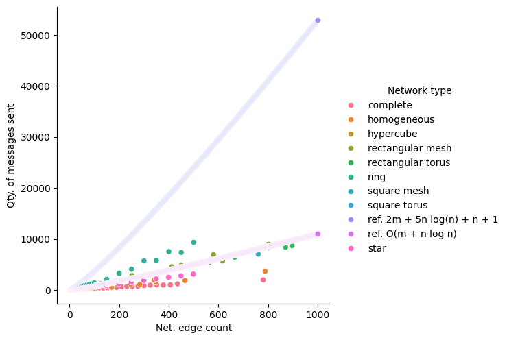
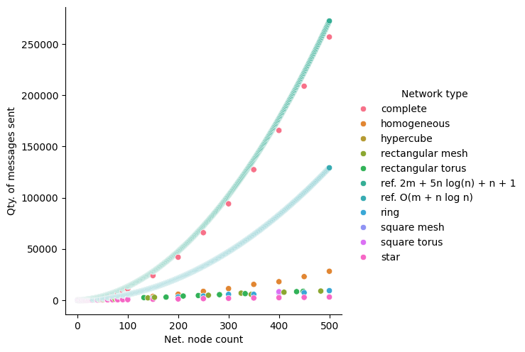
../../_images/notebooks_mega_merger_benchmarking_21_1.png

Again, we project the theoretical upper bound to a 2D space. Now the bound is a function of the number of nodes only.

[13]:

from math import log2

# restore the original results
benchmark_ideal.results = back.copy()

for n in range(1, 501):
    n = 1.0 * n
    m = n * (n - 1) / 2  # Maximum number of edges for any connected network with n nodes (a complete graph)

    loose_bound = m + n * log2(n)  # O(m + n log n)
    benchmark_ideal.results.insert(
        0,
        {
            "Net. node count": n,
            "Net. edge count": m,
            "Network type": "ref. O(m + n log n)",
            "Qty. of messages sent": loose_bound,
            "Qty. of messages delivered": loose_bound,
            "Qty. of status changes": loose_bound,
            "Qty. of steps": loose_bound,
        },
    )

    tight_bound = 2 * m + 5 * n * log2(n) + n + 1
    benchmark_ideal.results.insert(
        0,
        {
            "Net. node count": n,
            "Net. edge count": m,
            "Network type": "ref. 2m + 5n log(n) + n + 1",
            "Qty. of messages sent": tight_bound,
            "Qty. of messages delivered": tight_bound,
            "Qty. of status changes": tight_bound,
            "Qty. of steps": tight_bound,
        },
    )

Plot the results

[14]:

benchmark_ideal.plot_analysis(
    y_vars=[
        "Qty. of messages sent",
    ],
    x_vars=["Net. node count"],
    pairplot_kwargs={"height": 5},
)

[14]:

<seaborn.axisgrid.PairGrid at 0x7f15336cd7d0>

../../_images/notebooks_mega_merger_benchmarking_25_1.png

[15]:

# restore the original results
benchmark_ideal.results = back.copy()

Inferring time complexity

Let’s focus on the quantity of steps as a function of the number of nodes and edges.

[19]:

benchmark_ideal.plot_analysis(
    y_vars=["Qty. of steps"],
    pairplot_kwargs={"height": 5},
)

[19]:

<seaborn.axisgrid.PairGrid at 0x7f153fab0090>

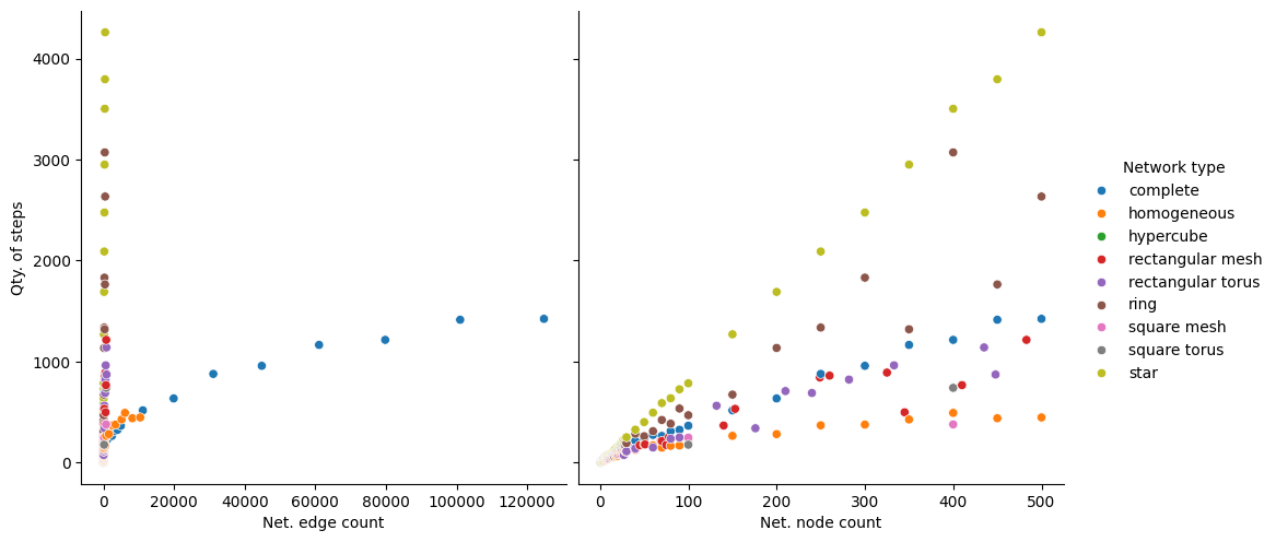
../../_images/notebooks_mega_merger_benchmarking_29_1.png

Since we are aiming to infer the worst time complexity of the algorithm, we must focus on the worst case scenario. This seems to be the case where the network is a ring:

[21]:

benchmark_ideal.plot_analysis(
    y_vars=["Qty. of steps"],
    result_filter=lambda line: line["Network type"] == "ring",
    pairplot_kwargs={"height": 5},
)

[21]:

<seaborn.axisgrid.PairGrid at 0x7f153fa84d50>

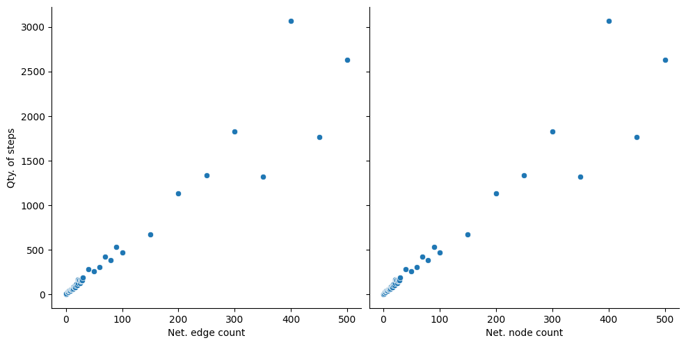
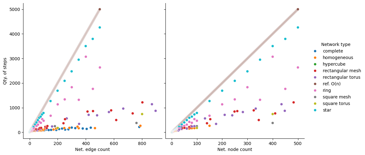
../../_images/notebooks_mega_merger_benchmarking_31_1.png

Obviously, the number of steps appears to be a linear function of the number of nodes and edges. Let’s plot a linear regression to confirm this.

[29]:

from math import log2

# restore the original results
benchmark_ideal.results = back.copy()

for n in range(1, 501):
    n = 1.0 * n
    m = n - 1

    loose_bound = m + n * log2(n)  # O(m + n log n)
    benchmark_ideal.results.insert(
        0,
        {
            "Net. node count": n,
            "Net. edge count": m,
            "Network type": "ref. O(n)",
            "Qty. of messages sent": n,
            "Qty. of messages delivered": n,
            "Qty. of status changes": n,
            "Qty. of steps": 10 * n,
        },
    )

[34]:

benchmark_ideal.plot_analysis(
    y_vars=["Qty. of steps"],
    result_filter=lambda line: line["Net. edge count"] < 1_000,
    pairplot_kwargs={"height": 5},
)

[34]:

<seaborn.axisgrid.PairGrid at 0x7f15563bf190>

../../_images/notebooks_mega_merger_benchmarking_34_1.png

Benchmarking: communication with delays

Now we will run a very similar battery of simulations, but with a delay in the communications. We will not analyze the results in detail again.

[35]:

benchmark_with_delay = AlgorithmBenchmark(
    ((MegaMergerAlgorithm, ExampleParameters.numerical_parameters),),
    network_behavior=NetworkBehaviorModel.RandomDelayCommunication,
    network_sizes=list(range(1, 15)) + list(range(15, 76, 10)) + list(range(100, 200, 50)),
    network_repeat_count=defaultdict(lambda: 1),
)

benchmark_with_delay.run()

[36]:

benchmark_with_delay.plot_analysis()

[36]:

<seaborn.axisgrid.PairGrid at 0x7f155cc80cd0>

../../_images/notebooks_mega_merger_benchmarking_37_1.png

[37]:

benchmark_with_delay.plot_analysis(
    result_filter=lambda line: line["Network type"] in ("complete", "homogeneous"),
    y_vars=["Qty. of messages sent", "Qty. of steps"],
)

[37]:

<seaborn.axisgrid.PairGrid at 0x7f15513a9150>

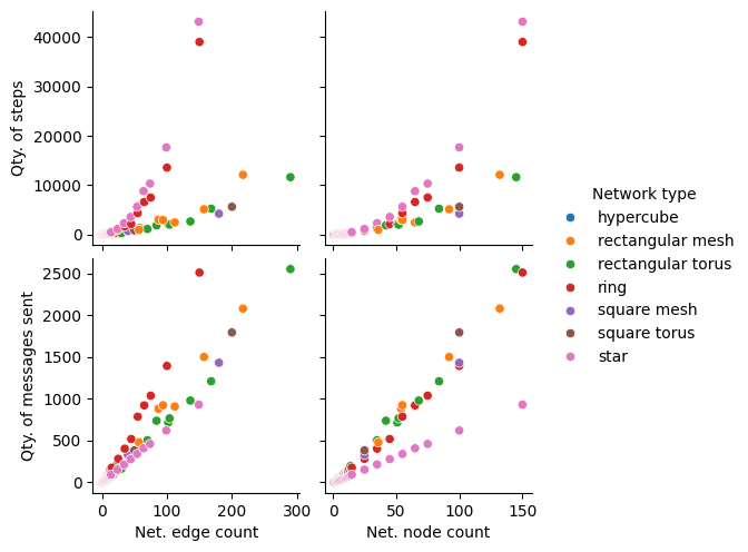
../../_images/notebooks_mega_merger_benchmarking_38_1.png

[38]:

benchmark_with_delay.plot_analysis(
    result_filter=lambda line: line["Network type"] not in ("complete", "homogeneous"),
    y_vars=["Qty. of messages sent", "Qty. of steps"],
)

[38]:

<seaborn.axisgrid.PairGrid at 0x7f15586f37d0>

../../_images/notebooks_mega_merger_benchmarking_39_1.png